Introduction to Neural Compression

Learned neural methods for lossy image compression

Desi R. Ivanova

Last updated on 18 Feb, 2022 7 min read ML

While searching for a research internship in industry, I discovered the exciting and rapidly growing field of neural data compression and decided to summarise what I’ve learned in this blog post. Specifically, I’ll give a brief introduction to neural-based approaches for lossy compression, mainly focusing on images, though the methods discussed can be applied to other data modalities too.

The compression pipeline

The typical compression pipeline consists of four components:

Encoding: input image $x$ is passed through an encoder function $\mathcal{E}$, transforming it into a latent representation $z$.
Quantisation: truncate $z$ to discard some of the least significant information.
Entropy coding: losslessly store the truncated latent $\hat{z}$ using some form of entropy coding (e.g. arithmetic coding).
Decoding: the original $x$ is reconstructed as $\hat{x}$, obtained by passing $\hat{z}$ through a decoder function $\mathcal{D}$.

Note that it is the quantization step that makes the compression lossy—the encoder can be a bijective function. We quantify the closeness between the original and the reconstructed image according to some distortion measure $d$, common choice for which is squared error $d(x, \hat{x}) = \lVert x - \hat{x}\rVert^2_2$.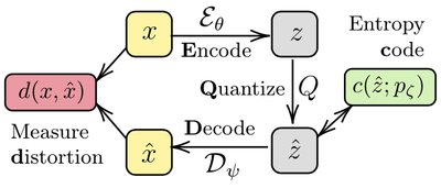

Main components of an image compression pipeline.

While the traditional compression approaches (e.g. JPEG) optimize each of these components independently, neural-based learned methods optimize them jointly, which can be hugely beneficial. Naturally, such neural approaches build upon autoencoder architectures and consist of three learnable components: encoder $\mathcal{E}_{\theta}$, decoder $\mathcal{D}_\psi$ and entropy model $p_\zeta$, where $\theta, \psi$ and $\zeta$ are trainable parameters.

Training objective

At its core, lossy compression is a trade-off between two metrics—distortion $d$ and bit rate $r$, determined by a Lagrange multiplier $\lambda$. Formally, we can write the objective function for the autoencoder as $$ \begin{aligned} L(\theta, \psi, \zeta) &= \underbrace{\mathbb{E}_{p(x)}\big[-\log p_\zeta( \hat{z} )\big]}_{\text{bit rate}} + \lambda \underbrace{\mathbb{E}_{p(x)}\big[ d(x, \hat{x})\big]}_{\text{distortion, set } d(x, \hat{x}) = \lVert x - \hat{x}\rVert^2_2} \\
& = \mathbb{E}_{p(x)}\Big[-\log p_\zeta(Q(\mathcal{E}_{\theta}(x))) + \lambda \lVert x - \mathcal{D}_\psi(Q(\mathcal{E}_{\theta}(x)))\rVert^2_2 \Big], \end{aligned} $$ where $p(x)$ is the (unknown) image distribution. We can approximate the expectation by sampling images from our training dataset, so it looks like we might be able to minimise $L$ using autodiff and standard stochastic gradient schemes. Unfortunately, the quantization component makes the objective non-differentiable and thus not easily opimisable in an end-to-end manner. One way around this problem is to continuously relax the objective which we discuss next.

Relaxed training objective and equivalence to VAEs

Ballé et al. (2017) replace the quantization step during training with additive uniform noise on the unit interval centred at $z$, i.e. $\hat{z} = Q(z)$ is substituted by $\tilde{z}$, sampled from a distribution $\tilde{z}|x \sim \mathcal{U}\big(\mathcal{E}_\theta(x)-1/2, \mathcal{E}_\theta(x)+1/2\big) =: q(\tilde{z}|x)$. The relaxed training objective can then be written as $$ \begin{aligned} L(\theta, \psi, \zeta) = \mathbb{E}_{p(x)q(\tilde{z}|x)}\big[-\log p_\zeta(\tilde{z}) + \lambda \lVert x - \mathcal{D}_\psi(\tilde{z})\rVert^2_2 \big]. \end{aligned} $$

Notice that $$ \log \mathcal{N} \left(x; \mathcal{D}_\psi(\tilde{z}), \frac{1}{2\lambda} \right) = - \lambda \lVert x - \mathcal{D}_\psi(\tilde{z})\rVert^2_2 + \text{const}, $$ so minimising the loss $L$ above is exactly equivalent to minimising $$ \begin{aligned} L(\theta, \psi, \zeta) = \mathbb{E}_{p(x)q(\tilde{z}|x)} \left[-\log p_\zeta(\tilde{z}) - \log \mathcal{N}\left(x; \mathcal{D}_\psi(\tilde{z}), \frac{1}{2\lambda} \right) \right]. \end{aligned} $$

Recall that VAEs (Kingma and Welling, 2014) are trained to minimize a KL divergence between a variational posterior $q(\tilde{z}|x)$ and the true posterior $p(\tilde{z}|x)$: $$ \begin{aligned} \mathbb{E}_{p(x)}\Big[ & KL \big(q(\tilde{z}|x) \lVert p(\tilde{z}|x) \big) \Big] = \mathbb{E}_{p(x)}\mathbb{E}_{q(\tilde{z}| x)}\left[ \log \frac{q(\tilde{z}; x)}{p(\tilde{z}|x)} \right] \\
&= \mathbb{E}_{p(x)}\mathbb{E}_{q(\tilde{z}| x)}\Big[ \log q(\tilde{z}| x) - \log p(x|\tilde{z}) - \log p_\zeta(\tilde{z}) +\log p(x) \Big] \\
&= \mathbb{E}_{p(x)} \underbrace{\Big[ - H(q(\tilde{z}| x))\Big]}_{=0} + \underbrace{\mathbb{E}_{p(x)}\mathbb{E}_{q(\tilde{z}| x)}\Big[ - \log p_\zeta(\tilde{z}) - \log p(x|\tilde{z}) \Big]}_{\equiv\text{relaxed rate-distortion objective}} + \text{const} \end{aligned} $$ If we choose a Gaussian distribution for the conditional likelihood of the observation, i.e. set $p(x|\tilde{z}) = \mathcal{N}\left(x; \mathcal{D}_\psi(\tilde{z}), 1 / 2\lambda\right)$, then we recover the relaxed rate-distortion objective.

To summarise, we have established that optimising rate-distortion trade-off (with fixed $\lambda$), using MSE as a distortion metric, is equivalent to training a VAE with Gaussian likelihood. In general, different choices of distortion metrics correspond to different distributions, though not all metrics give rise to a normalised density function. The rate corresponds to the negative log-prior, while distortion corresponds to the negative log-likelihood.

Why not use a simple autoencoder?

If you are new to the field of neural compression, you might be wondering (at least I was) why do we bother training a VAE. Indeed, recall that we introduced the uniform noise to deal with the non-differentiability of the quantization step. What if we simply skip quantization? A simple alternative compression pipeline would then be “encode an image $x$ into a low-dimensional latent representation $z$ and store that losslessly; at decompression time use a decoder to reconstruct $x$ from $z$", which would correspond to training a standard (i.e. not variational) autoencoder.

The reason why this procedure will not work is that $z$ being low-dimensional is not sufficient for efficient compression; what we require is $z$ to be low entropy. We can have a low-dimensional latent representation $z$, which is high entropy, and vice-versa—$z$ can be the same dimension as $x$ but much lower entropy, making it easy to compress losslessly. To ensure that the latent $z$ is low-entropy we need to be able to calculate that entropy, $H(z)=-\mathbb{E}_{p(z)}[\log p(z)]$, and to that end, we require the distribution $p(z)$. In other words, for efficient compression we require a full probabilistic model.

Side note: The entropy model $p_\zeta(z)$ corresponds to the prior in a VAE. In some applications, this prior is a fixed (simple) distribution, e.g. standard Gaussian, and its main role is to act as a regulariser. In neural compression settings the prior is learned and, as discussed above, is crucial for efficient compression. Indeed a lot of research has been focused on improving the entropy model—for example, Ballé et al. (2018) introduce a hyperprior. For a recent review on learned image compression see Hu et al. (2021).

How good are learned image compression models?

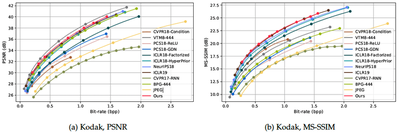
Learned image compression methods are competitive or outperforming traditional ones, such as JPEG and BPG, on the basis of standard performance metrics such as peak signal-to-noise ratio (PSNR) and multi-scale structural similarity index measure (MS-SSIM). The figure below is taken from Hu et al. (2021) and shows rate-distortion curves for different approaches.

Rate-distortion curves achieved by traditional methods (JPEG and BPG) neural-based learned approaches (all the rest) on the Kodak dataset. **Source**: Hu et al. (2021).

Challenges

The field of learnt image compression has undoubtedly made huge progress over the past few years. It is an active area of research, and many enhancements are being developed, e.g. better probabilistic models, better training objectives, per instance fine-tuning etc. However, two key challenges need to be addressed before these methods find their way into practice:

Computational cost: encoding and decoding can be too slow for practical applications.
Storage cost: encoder, decoder and entropy model typically have a lot of parameters, which could make them prohibitively expensive to store on end devices such as mobile phones.

References

Ballé J., V. Laparra, and E. P. Simoncelli, “End-to-end Optimized Image Compression”, in International Conference on Learning Representations (ICLR), 2017.

Ballé J., D. Minnen, S. Singh, S. J. Hwang, and N. Johnston, “Variational image compression with a scale hyperprior”, in International Conference on Learning Representations (ICLR), 2018.

Hu Y., W. Yang, Z. Ma, and J. Liu “Learning End-to-End Lossy Image Compression: A Benchmark”, IEEE transactions on pattern analysis and machine intelligence, 2021.

Kingma D. P., and M. Welling, “Auto-encoding variational Bayes”, arXiv preprint arXiv:1312.6114, 2013.