Towards more rigorous evaluations of language models
This is an extended and more thoughtful version of On Some (Fixable) Limitations of “Understanding the Limitations of Mathematical Reasoning in LLMs”. You can also read this on Substack.
1. Introduction
A staggering volume of research papers on (large) language models (LMs) is published daily. On the day of writing this (5th Nov 2024), 239 papers containing “LLM” or “Language Model” in their titles were added to the Computer Science section of arXiv alone. This flood of publications makes it difficult to separate genuine insights from noise, especially in areas lacking precise definitions, such as “reasoning”. Given the empirical nature of LLM research, much is open to interpretation, making rigorous analysis crucial to reduce bias and improve the reliability of findings.
In this post, we argue that LM researchers—especially those working in areas where core concepts lack established definitions—must adopt statistical methods to improve the rigor of their empirical evaluations. Leveraging techniques from classical statistics, such as confidence intervals and hypothesis tests, will help move the field beyond anecdotal observations and philosophical arguments toward a more scientific understanding of model behaviour.
To illustrate this in practice, we outline three key elements of rigorous empirical evaluation and apply them to Mirzadeh et al. (2024)—a recent paper that examines whether LMs perform “formal reasoning” or rely on “sophisticated pattern matching”.
2. Elements of Rigorous Empirical Evaluation
- Clear articulation of assumptions and consideration of alternative explanations.
- Quantification of uncertainty in results through appropriate statistical measures.
- Careful consideration of train-test overlap, with reasonable attempts to evaluate on “out-of-sample” datasets when possible.
If one does not give thought to what the data would be like under the assumption that one’s theory is false, one is likely reinforcing confirmation bias rather than establishing the validity of the theory. “Reproducibility, p-values, and type III errors: response to Mayo”, Philip B. Stark (2022)
The first step in rigorous evaluation is to clarify assumptions and explore alternative explanations. Experiments can often be designed in ways that unintentionally favour the hypothesis being tested. By being upfront about assumptions, questioning their validity, and investigating alternative explanations, researchers will improve the reliability and robustness of their conclusions.
In some sense it [the p-value] offers a first line of defence against being fooled by randomness, separating signal from noise […]. “It’s Not the P-Values’ Fault”, Yoav Benjamini (2016)
A second essential step is quantifying uncertainty, using tools such as error bars and confidence intervals, which help us gauge the reliability of performance metrics by providing a range of plausible values. Additionally, although often criticised, hypothesis tests and p-values can serve as an initial, coarse filter to distinguish signal from noise, laying the groundwork for deeper exploration into the practical significance of the reported results.
Finally, evaluating models on entirely unseen (“out-of-sample”) data is essential for accurately assessing their true capabilities. Unfortunately, identifying the extent of train-test overlap in LMs is both difficult and often neglected. Many language models are not transparent about this issue, and benchmark datasets frequently get leaked (or contaminated) during training, leading to biased evaluations and inflated performance metrics. As Zhang et al. (2024) highlight, reporting train-test overlap statistics is crucial for ensuring the validity of model evaluations.
To illustrate these three principles, we use Mirzadeh et al. (2024) as a case study—a recent paper that received substantial attention from the LLM research community with millions of views across social media platforms and the world-wide-web (e.g. see this, this, or this). We review their methods, identify gaps in their analysis, and offer a more rigorous statistical assessment of their claims.
Note: Whilst writing this blog post, a great overview of statistical methods suitable for evaluating LMs was published by Miller (2024).
3. Summary of Mirzadeh et al. (2024)
Mirzadeh et al. (2024) make two technical contributions: (1) a new benchmark, called GSM-Symbolic, for evaluating mathematical reasoning of LMs, and (2) an empirical evaluation of 25 LMs on this new benchmark to assess their reasoning capabilities.
3.1 What is the new benchmark and how is it constructed?
The authors propose GSM-Symbolic, a variant of the well-established GSM8K benchmark for grade school math word problems (Cobbe et al., 2021). Since GSM8K has likely leaked into many LMs' training sets due to its popularity, GSM-Symbolic aims to match its distribution whilst eliminating (or reducing) train-test overlap.
The authors also construct four variants of GSM-Symbolic by modifying question difficulty:
- GSM-M1: An easier version that removes one clause from each question.
- GSM-P1 and GSM-P2: Progressively harder versions that add one or two extra clauses respectively.
- GSM-NoOp: A version that adds “seemingly relevant but ultimately irrelevant information” that should have no operational significance (NoOp).
To generate GSM-Symbolic and the variants, the authors create “templates” from GSM8K questions by identifying modifiable variables whilst preserving the underlying logic. Each variable has a specified domain and constraints to ensure valid questions and answers. Here’s an example template:
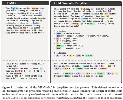
For their analysis, the authors select 100 questions from GSM8K and create such a template for each of them. Whilst the paper does not specify their selection method, we think that these questions were sampled randomly from GSM8K’s test set. By sampling values for the variables, 50 new questions are generated from each template. This means that GSM-Symbolic and each of its 4 variants (GSM-M1, GSM-P1, GSM-P2, and GSM-NoOp) contain 50 datasets of 100 questions each.
Throughout this post, when we refer to “GSM8K”, we specifically mean those 100 original GSM8K questions that were used to create the templates, not the full GSM8K dataset.
3.2 What are the key findings and conclusions from the empirical evaluation?
The evaluated model families include Gemma, Phi, Mistral and Llama (open weights), and GPT and o1 (proprietary, OpenAI). Of the open weights models, one can be considered “medium” size (Gemma2 27B params), and all the rest can be considered “small” (9B params or less). The metrics reported are average accuracy across the 50 versions of each dataset and the standard deviation of these accuracies.
The key findings are:
Performance variability: LMs exhibit some variability in performance across different instantiations of the same question.
Performance decline: Compared to GSM8K, performance on GSM-Symbolic drops, suggesting potential data contamination.
Sensitivity to question complexity: As complexity of the questions increases, “the performance [of models] decreases and the variance increases”, which is said to suggest that “models are not performing formal reasoning”, and that the increase in variance is “in line with the pattern-matching hypothesis”.
Impact of irrelevant information: Introducing a clause of no operational significance (NoOp), leads to large performance degradation across models, suggesting “deeper issues in their reasoning processes”.
The paper concludes that LMs “are not performing formal reasoning”.
4. Critical analysis and re-evaluation
Note 1: We provide a rigorous description of the mathematical framework which we use to analyse the results from Mirzadeh et al. (2024) in the Appendix.
Note 2: We run some additional small-scale experiments to provide empirical evidence for the claims we make in this post. We use two of the models that were evaluated in the paper: Llama-3-8B-Instruct and Phi-3.5-mini-Instruct. All code will be made available on GitHub.
4.1 Performance variability: Why is variability not (that) interesting?
As demonstrated, all models show a significant variance across different sets. […] It is noteworthy that this variation even occurs […]. Mirzadeh et al. (2024); emphasis added.
The authors emphasise the “non-negligible variance” in model performance across different GSM-Symbolic datasets, framing it as surprising. But is it?
4.1.1 When is variability not expected?
Variability would indeed be unexpected if each resampled question was effectively the same as the original. The implicit assumption here is that if an LM solves (or fails to solve) a given question once, it should always solve (or fail to solve) it when presented with the same problem but with different numbers. In other words, this assumes that LMs never make arithmetic mistakes—a very strong assumption that is not examined or addressed in the paper.
Is this assumption valid? For humans, it clearly is not. Even when solving the same problem with different numbers or subjects, humans can make (non-reasoning related) errors, such as arithmetic mistakes or copying a number incorrectly. The same applies to LMs.
We demonstrate this empirically by looking at the performance of LMs on a basic addition task with varying digit lengths (e.g. “What is 147 + 562?"). Consistent with prior literature (e.g. Muffo et al., 2023; Yuan et al., 2023), we find that as the numbers get larger, accuracy declines, thus showing that simple arithmetic is not perfectly reliable. We go beyond digit length and also consider how the number of carry operations affects performance on this simple addition task. The figure below illustrates how the probability of answering a question correctly is affected by the number of digits $d$ of the numbers being added and the number of carry operations involved in the sum.
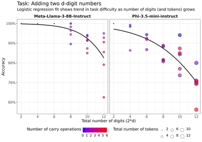
The regression results indicate that LM performance is negatively affected by both the number of digits and the number of carry operations in the sum. In other words, as the numbers get larger and the number of carry operations increases, accuracy declines. This suggests that LMs make errors similar to those made by humans, such as forgetting carry operations. Detailed regression results can be found in the Appendix.
Is performing arithmetic part of reasoning? Solving a math word problem consists of two steps: (1) translating the text to a sequence of operations, and (2) performing the operations correctly. Whilst the first step clearly requires reasoning ability, we argue that the second is more mechanical in nature and should not be considered as part of reasoning. To isolate “pure reasoning” capabilities, models could be provided with a calculator, which would help reduce (though not completely eliminate) the confounding effect of arithmetic errors.
4.1.2 When is variability expected?
If we (rightfully) reject the assumption that LMs are infallible in arithmetic, performance variability across datasets becomes entirely expected. Even if a model applies consistent reasoning, it may still make arithmetic errors, leading to natural performance variation.
How much variation is expected?
By now, it should be clear that the answer to this question depends on the assumptions we make about the data.
One reasonable assumption we could make is that each model $m=1, \dots, 25$, answers each question $n=1,\dots,100$ correctly with some probability $p_{m,n}$.
Unfortunately, since the paper does not provide question-level performance data, for the purposes of this analysis, we must further assume that this probability is constant across questions, that is $p_{m,n}=p_m$ for all $n$.
Thus, an LM answering questions is modelled as an independent and identically distributed Bernoulli trial with a model-specific success probability $p_m$. Under this assumption, the total number of correct answers on a dataset of size $N=100$ is $$Binomial(N, p_m).$$ The variance of this distribution is fully determined by the success probability $p_m$ and equals $$N \cdot p_m \cdot (1-p_m).$$ This variance is maximised when $p_m=1/2$ and goes to $0$ as $p_m$ approaches $0$ or $1$.
To understand what “expected” variation means under our assumption, we can construct confidence intervals (CIs) for the point estimates of $p_m$ on the GSM8K dataset. We highlight that the paper does not report such point estimates, but we can calculate the maximum likelihood estimates of $p_m$ by dividing the number of correct answers by the total number of questions. The number of correct answers (out of 100 questions) on the GSM8K questions are reported in the second column of Table 1 in the Appendix of the paper. We denote this estimate as $p^{8K}_m$ to indicate that it is computed from the GSM8K dataset.
There are different ways to construct CI for the Binomial proportion. The next figure shows Wilson score intervals, with more results included in the Appendix. To put this variability into perspective, we also include the average of the 50 point estimates for the model performance on GSM-Symbolic, which we denote as $p^{Symb}_m$.1
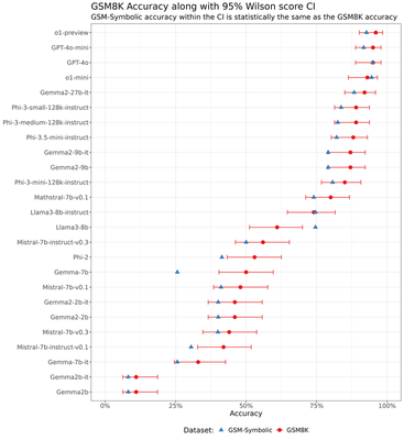
As expected, models with success probabilities closer to $1/2$ (e.g. Gemma-7b, Phi-2, Mistral-7b-v0.1) exhibit wider confidence intervals, reflecting higher variability. Conversely, models with success probabilities closer to 0 or 1 (Gemma2b, GPT-4o, o1-preview) have substantially narrower intervals.
Assuming that GSM8K and GSM-Symbolic come from the same distributions (more on that in Section 4.2.1), let’s look at Figure 2 of the paper.
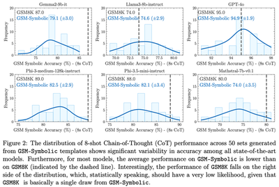
For the models shown in this figure, the GSM8K accuracy, $p_m^{8K}$, (represented by the dashed line) varies from 74% for the weakest model, Llama3-8B-instruct, to 95% for the strongest model, GPT-4o. The range of accuracies achieved on the 50 GSM-Symbolic datasets is relatively wide for Llama3-8B-instruct (approximately between 69% and 81%) and relatively narrow for GPT-4o (approximately between 91% and 98%). Importantly, for both models, the variation in GSM-Symbolic performance falls well within the Wilson score CIs of GSM8K performance that we calculated earlier! We visualise this in the next figure, showing the overlap between the 95% Wilson score CIs for $p^{8K}_m$ and the accuracy ranges on GSM-Symbolic for the models that had results reported in the paper (note that this does not include all 25 models).
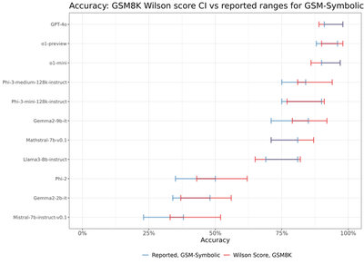
Note that our confidence intervals tend to be wider than the implied ranges in the figures in the paper, i.e. under the i.i.d. Bernoulli assumption, the expected variation is actually larger than what is observed. This discrepancy is likely to be explained by the unmodelled correlations between answers to questions coming from the same template—as initially suggested, a more reasonable assumption would be to model the probability of success on a template level, $p_{m,n}$, rather than assuming each questions arising from different templates are equally likely to be answered correctly. The analysis can be repeated once (if) the detailed question-level data becomes available.
Verdict: The observed variability in GSM-Symbolic performance is not inherently surprising, and we provide empirical evidence that it is indeed expected.
4.2 Performance decline on GSM-Symbolic
The paper claims that LMs perform worse on GSM-Symbolic compared to GSM8K. Let’s examine the evidence presented in Section 4.1, which we quote directly:
Another noteworthy observation is that the performance (represented by the dashed line in Fig. 2) on the original questions from the 100 examples of GSM8K used as templates is often more than one standard deviation away from the center of the GSM-Symbolic performance distribution, frequently on the right side of the distribution (this holds for 21 out of 25 models). One explanation for this could be data contamination […]. Mirzadeh et al. (2024); emphasis added.
There are two issues with the above quote. First, the authors suggest data contamination as one possible explanation for the performance decline, but do not explore other plausible explanations. Second, they rely on a hand-wavy “one standard deviation” criterion to suggest that the decline in performance is significant, without proper statistical analysis. We address both of these next.
4.2.1 Alternative explanation: Distribution mismatch
In addition to data contamination, another plausible explanation for the alleged performance discrepancy is a distribution mismatch between GSM8K and GSM-Symbolic. We note that the two explanations are not mutually exclusive—both can be true at the same time and should be evaluated appropriately.
The paper does not examine or discuss the potential distribution mismatch, making it impossible to draw definitive conclusions without access to the templates used. However, there is evidence indicating that the distribution of GSM-Symbolic questions differs from that of GSM8K, and that GSM-Symbolic is indeed more difficult. Looking at the example template (Figure 1 from the paper, reproduced above), we see that the sampling ranges for some variables exclude the original GSM8K values:
- The variable
totalis sampled from $(100, 500)$, whilst in the original question we havetotal=62. - The variable
ansis sampled from $(85, 200)$, whilst in the original question we haveans=14.
In other words, the original GSM8K question cannot be generated from the sampling ranges in the Symbolic template of Figure 1. In the next table, we propose more suitable ranges for all variables in the symbolic template, that ensure that the original question can be reproduced.
| Variable | Symbolic range | Proposed range (ours) | Original value |
|---|---|---|---|
total (toys) | $(100, 500)$ | $(10, 100)$ | $62$ |
x (building blocks) | $(5, 100)$ | $(4, 40)$ | $31$ |
y (stuffed animals) | $(5, 100)$ | $(1, 20)$ | $8$ |
z (stacking rings) | $(5, 100)$ | $(1, 20)$ | $9$ |
ans (bouncy balls) | $(85, 200)$ | $(4, 40)$ | $14$ |
The GSM-Symbolic sampling ranges for the variables from Figure 1 in Mirzadeh et al. (2024) (reproduced above) and our proposed sampling ranges. We highlight that the original GSM8K question cannot be generated from the proposed symbolic template because the symbolic ranges do not include the original values, whereas our proposed ranges do. We also believe that the proposed ranges better align with the context of the variables (e.g. having between 4 and 40 bouncy balls is more realistic than having between 85 and 200).
Since accuracy decreases as the number of digits in arithmetic operations increases (as discussed in Section 4.1.1), we expect that our proposed smaller ranges would result in higher accuracy compared to the original template, assuming that the reasoning process is executed correctly.
The question in Figure 1 involves three arithmetic operations: two additions and one subtraction. Assuming that subtraction is as difficult as addition, the probability of getting all three operations correct is the product of the individual probabilities of each operation being answered correctly.
To quantify the difference in accuracy that might arise from using the ranges in the paper versus the ranges we propose, we apply the logistic regression model from Section 4.1.1. Specifically, we consider the operations $(x+y)$, $(x+y)+z$, and $(x+y+z)+ans$ as the three operations to directly apply our model.
We present the results for Phi-3.5-mini-instruct and Llama3-8b-instruct in the next two tables, reporting the mean and standard deviation over 512 samples. For each example sampled from the corresponding ranges, we estimate the probabilities of correctly performing each arithmetic operation using our logistic regression model.
| Phi | $x+y$ | $(x+y)+z$ | $(x+y+z)+ans$ | All 3 operations |
|---|---|---|---|---|
| Symbolic | 0.949 $\pm$ 0.004 | 0.941 $\pm$ 0.008 | 0.920 $\pm$ 0.008 | 0.821 $\pm$ 0.013 |
| Proposed (ours) | 0.955 $\pm$ 0.007 | 0.954 $\pm$ 0.006 | 0.950 $\pm$ 0.004 | 0.866 $\pm$ 0.009 |
Results for Phi-3.5-mini-instruct model. Mean and standard deviation of probabilities over 512 examples.
| Llama | $x+y$ | $(x+y)+z$ | $(x+y+z)+ans$ | All 3 operations |
|---|---|---|---|---|
| Symbolic | 0.996 $\pm$ 0.001 | 0.995 $\pm$ 0.001 | 0.991 $\pm$ 0.002 | 0.982 $\pm$ 0.003 |
| Proposed (ours) | 0.997 $\pm$ 0.001 | 0.997 $\pm$ 0.001 | 0.996 $\pm$ 0.001 | 0.990 $\pm$ 0.001 |
Results for Llama3-8b-instruct model. Mean and standard deviation of probabilities over 512 examples.
For the Llama3-8b-instruct model, the smaller sampling ranges that we propose have a minimal effect: the probability of correctly performing all 3 operations is only $0.8$ percentage points higher compared to the symbolic ranges. In contrast, for the Phi-3.5-mini-instruct model, the effect is substantially larger: the probability of correctly performing all 3 operations is $86.6%$ with our proposed ranges, compared to $82.1%$ with the symbolic ranges—a difference of $4.5$ percentage points. Interestingly, this difference is similar to the performance drop observed for this model on the GSM8K vs the GSM-Symbolic datasets, which is $5.9$ percentage points ($88.0%$ on GSM8K vs $82.1%$ on GSM-Symbolic).
Based on the analysis for this question template, we argue that even if the models execute the “reasoning” process perfectly, i.e. they are able to correctly translate the math word problem into a sequence of arithmetic operations, they would still perform worse on the Symbolic template compared to our proposed template. Extrapolating from this, we suggest that if similar systematic discrepancies are present in other templates, then some (for some models likely substantial) portion of the observed performance decline could be attributed to an increased frequency of arithmetic errors.
Note: Using this analysis, we can conclude that the probability of successfully performing all arithmetic operations decreases exponentially as the number of arithmetic operations increases (more on this in Section 4.3).
Verdict: We provide some evidence for the existence of a distribution mismatch between GSM8K and GSM-Symbolic, which we believe should be further investigated. This mismatch could explain (some of) the performance discrepancies, and we offer some empirical support for this claim. Data contamination, as suggested by the authors, is also a plausible explanation, and is not mutually exclusive with distribution mismatch.
4.2.2 Considering each model independently: Is the decline in performance statistically significant?
For the purpose of this analysis, let’s assume that GSM8K and GSM-Symbolic datasets come from the same distribution.
For many models in Figure 2, the dashed line is in the right tail of the distribution. Additionally, Figure 3 of the paper, reproduced below, reports substantial performance decrease for many other models. So is the performance decline statistically significant, or could it be attributed to normal variation?
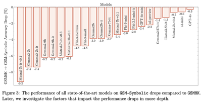
The right tool to determine whether these differences are statistically significant is hypothesis testing. For each model $m$, we want to test whether its success probability on GSM8K, denoted $p^{8K}_m$, equals its success probability on GSM-Symbolic, denoted $p^{Symb}_m$. This equality forms our null hypothesis. Our alternative hypothesis can take two forms:
- Two-sided alternative: The success probabilities are different
$$H_0: p^{8K}_m = p^{Symb}_m \quad\quad\quad H^{\text{two-sided}}_A: p^{8K}_m \neq p^{Symb}_m.$$
- One-sided alternative: The success probability on GSM8K is greater than that on GSM-Symbolic
$$H_0: p^{8K}_m = p^{Symb}_m \quad\quad\quad H^{\text{one-sided}}_A: p^{8K}_m > p^{Symb}_m.$$
We use Fisher exact test for the binomial proportion for all models, reporting the p-values in the next figure.
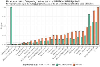
When analysing the models independently at the 5% significance level, we find that four models—Gemma-7b, Mistral-7b-instruct-v0.1, Phi-2, and Llama3-8b (indicated with (*) in the figure above)—exhibit statistically significant differences in performance based on the two-sided test. Among these four models, Llama3-8b performs statistically better on GSM-Symbolic compared to GSM8K, whilst the other three perform worse on GSM-Symbolic. The remaining 21 out of 25 models do not show a statistically significant difference in performance between GSM8K and GSM-Symbolic.
4.2.3 Considering all models together: Is the decline in performance statistically significant?
Although for most models there is no significant difference in performance, there is a trend that many models perform worse on GSM-Symbolic compared to GSM8K. To determine if this trend is statistically significant, we use the Wilcoxon signed-rank test, which is a non-parametric paired difference test.2
Before applying the test, we acknowledge two caveats and attempt to address them.
Caveat 1: Non-independent data. It is incorrect to perform the test on all 25 models because they are not independent. There are several types of dependence to consider. Most notably, base models and their instruct-tuned versions are related (e.g., Gemma2-9b and Gemma2-9b-it). Additionally, we believe that different sizes within the same model family are not independent (e.g., mini-small-medium for Phi or 2b-9b-27b for Gemma). Minor version updates (e.g., Mistral v0.1 vs. 0.3, Phi 3 vs. 3.5) are also likely correlated. So, although we have a sample of 25 models, the effective sample size is much smaller.
To address this, we have attempted to create sets of independent models and perform the test on these subsets. In each model family, we selected the latest, largest instruct-tuned version and repeated this process by also selecting the smallest version. This gives us two sets of 7 models, with differences between the two sets indicated in italics:
Subset of largest models: Gemma2-27b-it, Phi-3.5-mini-instruct, Mistral-7b-instruct-v0.3, Mathstral-7b-v0.1, Llama3-8b-instruct, GPT-4o, o1-preview.
Subset of smallest models: Gemma2-2b-it, Phi-3.5-mini-instruct, Mistral-7b-instruct-v0.3, Mathstral-7b-v0.1, Llama3-8b-instruct, GPT-4o-mini, o1-mini.
Caveat 2: Different sample sizes. We note that the success probability on GSM8K is estimated from only one sample (of 100 questions) and the success probability on GSM-Symbolic is estimated from 50 samples (each containing 100 questions). Whilst the test is valid, inaccurate measurements of the estimated success probabilities would lead to invalid conclusions.
Let’s define the vectors of success probabilities on GSM8K and GSM-Symbolic as
$$ p^{8K}_\text{subset}=[p^{8K}_1,\dots,p^{8K}_7] $$
and
$$ p^{Symb}_\text{subset}=[p^{Symb}_1,\dots,p^{Symb}_7], $$
respectively, where the subscript $\text{subset}\in{\text{largest},\text{smallest}}$. As before, we perform one-sided and two-sided tests:
Two-sided: The success probabilities are different $$ H_0: p^{8K}\text{subset} = p^{Symb}\text{subset} \quad\quad\quad H_A^\text{two-sided}: p^{8K}\text{subset} \neq p^{Symb}\text{subset}. $$
One-sided: The success probability on GSM8K is greater than that on GSM-Symbolic $$ H_0: p^{8K}\text{subset} = p^{Symb}\text{subset} \quad\quad\quad H_A^\text{one-sided}: p^{8K}\text{subset} > p^{Symb}\text{subset}. $$
The results of the hypothesis tests are given in the following table:
| Subset of Models | Two-sided p-value | One-sided p-value |
|---|---|---|
| Largest | 0.047 | 0.023 |
| Smallest | 0.078 | 0.039 |
Results of the Wilcoxon signed-rank test for the two subsets of models. At the 5% significance level, there is evidence of statistically significant differences in performance between GSM8K and GSM-Symbolic.
For the largest subset of models, both tests show statistically significant differences (at the $5%$ significance level but not at the $1%$ level), indicating that GSM8K outperforms GSM-Symbolic in the one-sided test. When looking at the smallest subset of models, the evidence for significant differences is somewhat weaker.
It is important to note that rejecting the null hypothesis, gives us strong evidence that the models perform worse on GSM-Symbolic, but does not imply that the models lack reasoning abilities. As mentioned in Section 4.2.1, the observed performance differences could also be due to distributional differences (for which there is substantial evidence), data contamination, or a combination of both.
Verdict: When analysing the results of models individually, there is little evidence of performance differences: out of 25 models, only 3 perform significantly worse on GSM-Symbolic compared to GSM8K, and 1 performs better. When we analyse the results of models together, we find some, albeit weak, evidence that the models perform worse on GSM-Symbolic. These differences could be due to several factors, including distribution mismatch, data contamination, or lack of reasoning capabilities.
4.3 Performance decrease and variance increase with question complexity
Mirzadeh et al. (2024) highlights the fact that performance decreases and variance increases with question complexity on multiple occasions, most notably in Section 4.3. Some examples include:
[page 3] We show that performance degradation and variance increase as the number of clauses increases, indicating that LLMs’ reasoning capabilities struggle […]
[page 9, Figure 6 reproduced below] the distribution of performance shifts to the left (i.e., accuracy decreases), and the variance increases.
[page 9] the increase in variance suggests that searching and pattern-matching become significantly harder for models as the difficulty increases.
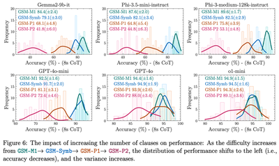
The figure above shows the results for four datasets: the baseline GSM-Symbolic, GSM-M1 (Minus 1), which removes a clause, and GSM-P1 (Plus 1) and GSM-P2 (Plus 2), which add one and two clauses respectively. It is reasonable to expect that a model will perform better on easier datasets and worse on more difficult ones. As before, we assume that a model $m$ answers questions of varying difficulty levels $\text{dif}=-1, 0, 1, 2$ as independent and identically distributed Bernoulli trials with a success probability of $p^\text{dif}_m$. The distribution of the total number of correct answers follows a binomial distribution $Bin(N=100, p^\text{dif}_m)$, with variance equal to $N \cdot p^\text{dif}_m \cdot (1 - p^\text{dif}_m)$.
If the probabilities of success decrease with increasing question complexity, i.e. $p^\text{dif=-1}_m > p^\text{dif=0}_m > p^\text{dif=1}_m > p^\text{dif=2}_m > 0.5$, the corresponding variances must increase.3 We believe that this is precisely what we observe in Figure 6: the increase in variance is a trivial consequence of the decrease in probabilities of success, rather than a sign of “pattern-matching” becoming harder.
Regarding the decrease in probability of success itself, it is plausible that reasoning becomes more challenging as additional clauses are introduced, or conversely, easier when clauses are removed, as seen in the M1 template. Importantly, as noted in Section 4.2.1, introducing more clauses necessarily involves more arithmetic operations, which in turn will result in an exponential decline in performance. This decline will occur even if the models perfectly execute the “reasoning” process of translating the math word problem into a sequence of arithmetic operations. To distinguish between these two effects, a more detailed and thorough analysis will be needed.
We hypothesise that another reason for the decrease in performance could be the increasing length of the questions and the chain of thoughts required to solve them.4 Whilst models can of course handle longer contexts by utilising various context length extension techniques, past research suggests that performance tends to degrade when we go beyond the training context length.
Verdict: The emphasis on “non-negligible variance” and “increase in variance” throughout the paper appears to be an over-interpretation of expected statistical artifacts. The decrease in probability of success as question complexity increases can be due to both increased difficulty in reasoning and increased probability of making an arithmetic mistake.
4.4 Performance decline on the NoOp dataset
All models perform substantially worse on the NoOp dataset compared to GSM8K, as shown in Figure 8 (a) of the paper:
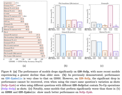
We repeat the independent and paired tests and indeed find that all models perform significantly worse on the NoOp dataset compared to GSM8K.
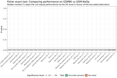
| Subset of Models | Two-sided p-value | One-sided p-value |
|---|---|---|
| Largest | 0.016 | 0.008 |
| Smallest | 0.016 | 0.008 |
The NoOp results present the most interesting results from the point of view of reasoning vs pattern-matching debate. For example, the results in Figure 8 (b) and (c) might suggest that the models in fact struggle to pattern-match (in context) as there is no signficiant improvement in performance when NoOp examples are provided in context. We believe there is scope for a range of ablations, such as prompting the model that “not all information might be relevant,” to gain deeper understanding of reasoning capabilities.
5. Conclusion
There’s huge value in developing new benchmarks and we believe that the proposed GSM-Symbolic can be quite useful!
The accompanying analysis, however, can be substantially improved with the help of basic statistics.
The frequentist approach we adopt here is particularly well-suited, as the Symbolic templates allow us to generate an arbitrary number of new datasets
Key findings from each subsection are summarised below:
[Section 4.1] We discussed the assumptions under which variability of performance on GSM-Symbolic is unexpected vs expected and quantifiable. We provided empirical evidence that variability is indeed expected.
[Section 4.2] We argued that distribution mismatch between the GSM8K and GSM-Symbolic datasets may explain some of the observed performance decline of models (in addition to contamination and “lack of reasoning”). We also quantified the extent to which the performance degradation on GSM-Symbolic is actually statistically significant. Considering models individually, only 3 out of 25 models show a statistically significant performance decline on GSM-Symbolic (and 1 performs significantly better). Taken together, there is some evidence for a performance decline on GSM-Symbolic vs GSM8K.
- [Section 4.3] The observed increase in performance variance with rising question complexity is likely an over-interpretation of expected statistical artefacts. The decrease in success probability as complexity grows can be attributed to both increased reasoning difficulty and a higher likelihood of arithmetic errors.
- [Section 4.4] The performance decline on the GSM-NoOp dataset is highly statistically significant. We believe that investigating the NoOp results in more detail could provide genuine insights into the models' reasoning capabilities.
Final thoughts: We strongly believe that without a rigorous statistical framework, there is a substantial risk of over-interpreting results and drawing misleading conclusions.5 We hope that this blog post can serve as a tutorial and can help researchers to get into the habit of thinking about and performing proper statistical evaluations of LLMs!
Appendix
Mathematical setup
Here we more rigorously describe the mathematical lens which we use to analyse the results from
- We sample a template $T$ from some distribution $\mathbb{P}_T$.
A template here is defined in the sense of
, that is, it is a mathematical word problem, in which numerical values (e.g. number of toys) and certain other objects (e.g. names of people) are marked as variables, to be filled-in later. - The template $T$ gives rise to a conditional distribution $\mathbb{P}_{V \vert T}$ over the admissible filler-values. We sample a set of such filler-values $V \sim \mathbb{P}_{V \vert T}(\cdot \vert T)$ and plug them into the template, producing a pair of a question and an answer $(T(V)_Q, T(V)_A)$.
We are interested in whether a language model $m$ answers a question correctly. We model this with the random variable $X_m$, defined as $$X_m = \mathbb{I}(m(T(V)_Q) = T(V)_A),$$ where $\mathbb{I}$ is the indicator function. The accuracy of model $m$, denoted as $p_m$, is then the expected value of $X_m$, i.e., $p_m = \mathbb{E}[X_m]$. The variable $X_m$ follows a $Bernoulli(p_m)$ distribution.
In fact, since we care about the difference in model performance on GSM8K and GSM-Symbolic, we postulate that we have two random variables $V^{8K}$ and $V^{Symb}$, governed by two conditional distributions: $\mathbb{P}^{8K}_{V|T}$, corresponding to GSM8K, and $\mathbb{P}^{Symb}_{V|T}$, corresponding to GSM-Symbolic. These two distributions may be the same or different.
This setup can be represented by the following directed probabilistic graphical model:
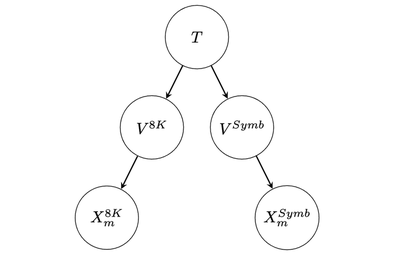
where, for the purpose of this analysis, the bottom-most arrows denote deterministic dependencies.
Under this model, we have $X_m^{8K} \sim Bernoulli(p_m^{8K})$ and $X_m^{Symb} \sim Bernoulli(p_m^{Symb})$, where $p_m^{8K}, p_m^{Symb} \in [0, 1]$ are our main parameters of interest.
In this framework, we can describe the experimental setup of Mirzadeh et al. (2024)
Templates $T$: 100 templates $t_1, t_2, \dots, t_{100}$ sampled independently from $\mathbb{P}_T$
Filler-values $V^{8K}$: one sample $v^{8K}_i$ from each conditional
$$\mathbb{P}^{8K}_{V \vert t_i} \quad \text{for} \quad 1 \le i \le 100$$
- Filler-values $V^{Symb}$: 50 i.i.d. samples $v^{Symb}_{i,j}, 1 \le j \le 50$ from each conditional
$$\mathbb{P}^{Symb}_{V | t_i} \quad \text{for} \quad 1 \le i \le 100$$
- Observed data: for each of these sets of filler-values and each model $m$ (in a pre-determined set of 25 language models), we have corresponding observations $$ \begin{aligned} x^{8K}_{m,t_i} \quad \text{and} \quad x^{Symb}_{m,t_i,j} \end{aligned} $$ for the GSM8K questions and the GSM-Symbolic questions—that is, whether model $m$ answered correctly the questions $$ \begin{aligned} t_i(v^{8K}_i) \quad \text{and} \quad t_i(v^{Symb}_{i,j}), \end{aligned} $$ respectively.6
- Accuracy estimates: from these observations, maximum likelihood estimates can be computed as $$ \begin{aligned} \hat{p}_m^{8K} = \frac{1}{100}\sum_{i=1}^{100} {x^{8K}_{m,t_i}} \end{aligned} $$ and $$ \begin{aligned} \hat{p}_{m, j}^{Symb} = \frac{1}{100}\sum_{i=1}^{100} x^{Symb}_{m,t_i, j}, ; 1 \leq j \leq 50 \end{aligned} $$
We note that only $\hat{p}_m^{8K}$ and the average $\overline{\hat{p}_m^{Symb}}=\frac{1}{50}\sum_{j=1}^{50}\hat{p}_{m,j}^{Symb}$ are reported in the paper (Table 1, Appendix A.2 in Mirzadeh et al. (2024)).
Under the assumptions of this mathematical model, we can think of $\hat{p}_m^{8K}$ as an observation from a random variable $$ \begin{aligned} \hat{P}^{8K}_m\sim\frac{1}{100}Bin(100,p^{8K}_m). \end{aligned} $$ Similarly, each $\hat{p}_{m,j}^{Symb}, 1 \le j \le 50$ is an observation of $$ \begin{aligned} \hat{P}^{Symb}_m\sim\frac{1}{100} Bin(100,p^{Symb}_m). \end{aligned} $$ We can’t assume that these observations are independent, due to the shared templates.
In this blogpost, the main question we’ve tackled is: given these observed $\hat{p}_m^{8K}$ and $\overline{\hat{p}_m^{Symb}}$, what evidence is there to believe that $p^{8K}_m \neq p^{Symb}_m$ or that $p^{8K}_m > p^{Symb}_m$?
Clopper-Pearson confidence intervals
For robustness purposes, here are the Clopper-Pearson confidence intervals for the point estimates of $p_m$:

The Clopper-Pearson CIs are slightly wider than those obtained using the Wilson score. Using Clopper-Pearson would not have changed any of the results (qualitative or quantitative) presented in this post.
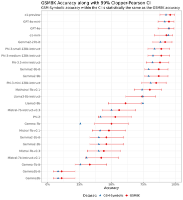
99% Confidence intervals
For completeness, we include 99% confidence intervals for the point estimates of $p_m$:

Logistic regression: full results
The logistic regressions were conducted in R (glm) on Posit Cloud.
Llama-3-8B-Instruct
Call:
glm(formula = correct ~ total_digits + carry, family = "binomial",
    data = .)

Coefficients:
             Estimate Std. Error z value Pr(>|z|)
(Intercept)   7.35210    0.47409  15.508  < 2e-16 ***
total_digits -0.41672    0.04859  -8.576  < 2e-16 ***
carry        -0.21252    0.07575  -2.806  0.00502 **
---
Signif. codes:  0 ‘***’ 0.001 ‘**’ 0.01 ‘*’ 0.05 ‘.’ 0.1 ‘ ’ 1

(Dispersion parameter for binomial family taken to be 1)

    Null deviance: 1125.63  on 3066  degrees of freedom
Residual deviance:  922.02  on 3064  degrees of freedom
AIC: 928.02

Number of Fisher Scoring iterations: 7
Phi-3.5-mini-Instruct
Call:
glm(formula = correct ~ total_digits + carry, family = "binomial",
    data = .)

Coefficients:
             Estimate Std. Error z value Pr(>|z|)
(Intercept)   3.95149    0.17593  22.460   <2e-16 ***
total_digits -0.25747    0.02249 -11.447   <2e-16 ***
carry        -0.02325    0.04907  -0.474    0.636
---
Signif. codes:  0 ‘***’ 0.001 ‘**’ 0.01 ‘*’ 0.05 ‘.’ 0.1 ‘ ’ 1

(Dispersion parameter for binomial family taken to be 1)

    Null deviance: 2460.8  on 3066  degrees of freedom
Residual deviance: 2217.8  on 3064  degrees of freedom
AIC: 2223.8

Number of Fisher Scoring iterations: 5
Computational resources
The extra experiments in this blog post (the addition task discussed in Section 4.1.1) were performed on a single L4 GPU (24GB VRAM) on a Lightning AI Cloud instance. The statistical analysis (confidence intervals, p-values) was performed on a laptop.
Similarly to $p^{8K}_m$, we obtain maximum likelihood estimates of $p^{Symb}_m$ from the average accuracy on GSM-Symbolic, reported in Table 1 of the paper. ↩︎
The careful reader would notice that in the previous subsection, we used parametric tests. This was because we do not have access to question-level data which is necessary for a non-parametric test. We would prefer non-parametric tests as they do not rely on distributional assumptions. ↩︎
We note that the average success probability on GSM-P2, $p^{\text{dif}=2}_m$, does fall below 0.5 for the models in the first row of Figure 6. Our point is still valid in these cases since $p^{\text{dif}=2}_m$ is closer to 0.5 than $p^{\text{dif}=1}_m$ and hence the variability on GSM-P2 is still expected to be larger than on GSM-P1. We would expect to see decrease in variance in cases where $0.5 > p^{\text{dif}=-1}_m > p^{\text{dif}=0}_m > p^{\text{dif}=1}_m > p^{\text{dif}=2}_m$. ↩︎
For example, the Phi-mini series of models has a default context length of 4K tokens (Abdin et al., 2024). ↩︎
Neither the Frequentist nor the Bayesian religion is perfect, but neglecting statistical analysis altogether would be the worst outcome. ↩︎
We note that this raw data is not made publicly available. ↩︎