Introduction to Bayesian Optimal Experimental Design

What questions should we ask in an online survey? Which point should we query next in an active learning loop? Where should we place sensors, e.g. to detect faults and defects most efficiently? These, and many more, seemingly distinct questions constitute the same fundamental problem—designing experiments to collect data that will help us learn about an underlying process. Bayesian Optimal Experimental Design (BOED) is a powerful yet elegant mathematical framework for tackling such problems. This introductory post describes the BOED framework and highlights some of the computational challenges of deploying it in applications. For an extensive review, see Ryan et al. (2016).

In the BOED framework, the relationship between the parameters $\theta$ of the underlying process, the controllable designs $\xi$, and the outcomes $y$ are described using a likelihood function (or simulator) $p(y|\xi, \theta)$. Our initial knowledge or beliefs about the parameters $\theta$ are encapsulated in a prior $p(\theta)$.

We assume $p(\theta)$ and $p(y|\theta, \xi)$ as given, so our task is to choose experiments $\xi$ that enable us to learn about $\theta$ as efficiently as possible. One possible measure of efficiency is the Expected Information Gain (EIG), proposed by Lindley (1956). Indeed, the guiding principle in BOED is that of information maximisation, and EIG is the central quantity of interest, so we introduce it below in detail.

Information Gain and Expected Information Gain (EIG)

To build some intuition, let’s begin with the illustrative example in Figure 1. Suppose we perform an experiment $\xi_1$ and obtain an outcome $y_1$. We compute the resulting posterior $p(\theta| \xi_1, y_1) \propto p(\theta) p(y|\theta, \xi)$ and notice that it is not very different from the prior; in particular, our uncertainty about $\theta$ is almost as large as before conducting the experiment (Figure 1, Left). Performing the experiment $\xi_2$, on the other hand, gives a posterior that is much more peaked, suggesting that $\xi_2$ is the more useful, more informative experiment of the two (Figure 1, Right).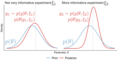

Formally, we quantify the information gain (IG) of an experiment as the reduction in Shannon entropy from the prior to the posterior $$ \text{IG}(\xi, y) = H\big[ p(\theta) \big] - H \big[ p(\theta | y, \xi) \big]. $$ Using this metric, we can now compare and rank design-outcome pairs; for example, we can say the pair $(\xi_2, y_2)$ is more informative about $\theta$ than $(\xi_1, y_1)$. However, we can’t use IG to find the optimal design as it depends on the outcome $y$ and hence can’t calculate it until after the experiment has been performed. An easy way to fix that is to take the expectation with respect to all possible outcomes $y$ for an experiment $\xi$, which defines the expected information gain $$ \text{EIG}(\xi) = \mathbb{E}_{p(y|\xi)}[\text{IG}(\xi, y)], $$ where $p(y|\xi) = \mathbb{E}_{p(\theta)} \big[ p(y|\theta, \xi) \big]$ is the marginal distribution of $y$. The optimal design is then $\xi^* = \arg\max_\xi \text{EIG}(\xi)$

Unfortunately, optimising the EIG is an extremely challenging task. In fact, even computing $\text{EIG}(\xi)$ for a fixed $\xi$ is very computationally costly, as both the posterior $p(\theta | y, \xi)$ and the marginal $p(y|\xi)$ are in general intractable (i.e. not known in closed form). How to deal with these intractabilities will be the topic of another post. For now, we assume that there are computational methods that allow us to estimate and optimise the EIG efficiently.

Multiple experiments

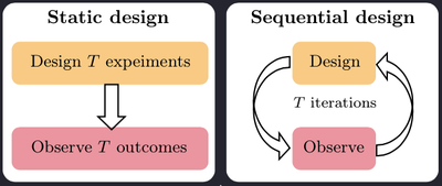
More often than not, we wish to perform multiple experiments $\xi_1, \xi_2, \dots, \xi_T$. Broadly speaking, there are two ways to approach the problem of designing multiple experiments: static (aka batch or open-loop) and sequential (aka adaptive or closed-loop).

Static experimentation

Instead optimising $\text{EIG}(\xi)$ with respect to a single design $\xi$, we can set $\underline{\xi} := (\xi_1, \xi_2, \dots, \xi_T)$ and optimise $\text{EIG}(\underline{\xi})$ to give us an optimal batch of designs. Static design strategies are useful when experiments need to be performed in parallel, which can be suitable, for example, in applications where it takes a long time to obtain the outcomes after the experiment has been performed. As a result, the outcome of any experiment cannot affect the design of the other experiments.

Sequential experimentation

In practice, we are often more interested in performing multiple experiments in a sequence $\xi_1, \xi_2, \dots, \xi_T$, and allowing the choice of each design $\xi_{t+1}$ to be guided by the data from past experiments, which we call the history and denote by $h_t:= (\xi_1, y_1, \dots, \xi_t, y_t)$.

Myopic design (one-step lookahead)

The traditional approach to designing adaptive experiments is to fit a posterior $p(\theta| h_t)$ and use that as a prior in the EIG optimisation, which would give the next design $\xi_{t+1}$. This is known as greedy or myopic design strategy: at each step of the experiment, we are optimising for the next best choice of $\xi$, without taking into account that there are $T-1$ future experiments to be performed. Despite being suboptimal, the sequential myopic strategy can bring huge improvements over static designs.

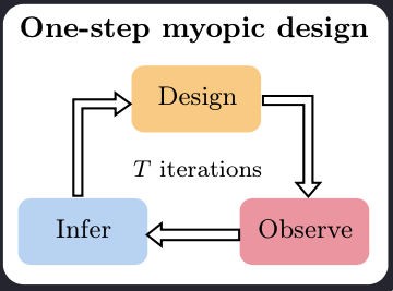
Unfortunately, the computational cost required to run the myopic strategy severely limits its applicability. At each stage $t+1$ of the experiment, we need to perform compute (or rather approximate) the posterior $p(\theta|h_t)$, which is expensive and cannot be done in advance as it depends on $y_{1:t}$. Furthermore, to obtain $\xi_{t+1}$, we need to maximise the EIG, which is computationally even more challenging. Both of these steps need to be performed during the live experiment. Unless we are dealing with unusually simple models, it will be infeasible to run the myopic (or non-myopic $K$-step lookahead) strategy in real-time experiments.

Amortized sequential BOED

Until recently, to perform BOED in real-time applications, one had to forego adaptivity and use static strategies instead. (Or alternatively, forego being Bayesian optimal and use an adaptive heuristic).

Deep Adaptive Design (DAD, Foster et al. 2021) is a method developed by our group at Oxford that has opened the door to running adaptive BOED in real-time. At the heart of the DAD approach is a design policy network, which is trained prior to the live experiment. The network takes a history $h_t$ as an input and outputs the design $\xi_{t+1}$ to be used for the next experiment. Design decisions are thus made in milliseconds, using a single forward pass through the network.

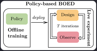
The key methodological difference, which marks a critical change from previous BOED approaches, is that DAD learns a policy, instead of learning designs. Put differently, previous methods optimise individual designs, while DAD optimises the parameters of a neural network, which is trained to propose optimal designs. DAD is thus the first policy-based approach to BOED.

To be able to train the design network, we addressed some major technical challenges, including formulating a unified training objective that doesn’t require calculating intermediate posteriors and EIGs, introducing a tractable surrogate for that objective and suggesting an appropriate architecture for the design network.

I’ll probably write another blog post to talk about our work on policy-based BOED at greater length. In the meantime, if you’re interested in learning more about DAD, you can watch our ICML talk or have a look at the full paper.

References

Foster A., D. R. Ivanova, I. Malik, and T. Rainforth, “Deep adaptive design: Amortizing sequential Bayesian experimental design”, International Conference on Machine Learning (ICML), 2021.

Lindley D. V., “On a measure of the information provided by an experiment”, The Annals of Mathematical Statistics, pages 986–1005, 1956.

Ryan E. G., C. C. Drovandi, J. M. McGree, and A. N. Pettitt, “A review of modern computational algorithms for Bayesian optimal design”, International Statistical Review, 2016.